Monday, October 13, 2008 Activity 20: Neural Networks Pattern recognition simply is making the computer recognize patterns we recognize visually. This begs the question: why not model pattern recognition the way our brain works? And this is what neural networks is about. Neural networks are composed of neurons arranged in a layer that is fully connected with the preceding layer. The layers are called the input, hidden and output layers respectively. The input layer is where the input features are fed and directed to the hidden layer which is again directed to the output layer. Neurons pass information using an "all-or-nothing" approach which is dependent on the strength of its connection to adjacent neurons.The tansig function is one of the most often used activation functions is pattern recognition problems. For neural networks I used MATLAB instead of Scilab since MATLAB has an inbuilt Neural Networks toolbox while Scilab needs ANN. I used the parameters from Activity 18 for the 4 classes of images which are: Area, Height over Width, Average R, and Average G. Below is the code I used: training = [5345 1.000000 0.758862 0.129754 6128 0.958763 0.756430 0.136960 5541 1.011494 0.814644 0.108821 1239 1.076923 0.602028 0.283912 1224 1.078947 0.629195 0.280192 1206 1.108108 0.611142 0.289349 439 0.444444 0.253336 0.508687 368 0.304348 0.248109 0.521104 372 0.444444 0.255933 0.518223 2080 1.000000 0.520683 0.374020 2064 1.040000 0.529217 0.382716 1977 1.083333 0.582884 0.345742 ]'; test = [ 5421 1.000000 0.795391 0.112691 5162 0.932584 0.826950 0.100648 5281 1.098765 0.788015 0.122597 1264 1.051282 0.633988 0.271862 1179 1.105263 0.618832 0.278147 1191 1.105263 0.615691 0.280110 306 0.409091 0.243423 0.517028 297 0.304348 0.245041 0.518146 304 0.239130 0.252019 0.514459 2000 0.980000 0.499452 0.372944 1956 1.020408 0.525111 0.379350 1906 1.062500 0.522208 0.392979 ]'; training_out = [0 0; 0 0; 0 0; 0 0; 0 1; 0 1; 0 1; 0 1; 1 1; 1 1; 1 1; 1 1]'; net=newff(minmax(training),[25,2],{'tansig','tansig'},'traingd'); net.trainParam.show = 50; net.trainParam.lr = 0.01; net.trainParam.lr_inc = 1.05; net.trainParam.epochs = 1000; net.trainParam.goal = 1e-2; [net,tr]=train(net,training,training_out); a = sim(net,training); a = 1*(a>=0.5); b = sim(net,test); b = 1*(b>=0.5); diff = abs(training_out - b); diff = diff(1,:) + diff(2, :); diff = 1*(diff>=1); Again, 100% classification was observed. Acknowledgments Thanks to Jeric for helping me with the code. I understood this activity! i give myself 10/10 neutrinos! posted by poy @ 2:43 AM   1 comments Activity 19: Linear Discriminant Analysis Moving on to our discussion about pattern recognition we study Linear Discriminant Analysis or LDA. Here we create a discriminant function from predictor variables. Here I tried classifying 5 centavo and 25 centavo coins. This time since both are (should be) circular, I remove the parameter of Height over Width leaving three parameters for classifications: Area, R (NCC) and G (NCC). The code I used is shown below: x = [1239 0.602028 0.283912; 1224 0.629195 0.280192; 1206 0.611142 0.289349; 2080 0.520683 0.374020; 2064 0.529127 0.382716; 1977 0.582884 0.345742]; xt = [1264 0.633988 0.271862; 1179 0.618832 0.278147; 1191 0.615691 0.280110; 2000 0.499452 0.372944; 1956 0.499452 0.379350; 1906 0.522208 0.392979];//Test class y = [1; 1; 1; 2; 2; 2;]; x1 = [1239 0.602028 0.283912; 1224 0.629195 0.280192; 1206 0.611142 0.289349]; x2 = [2080 0.520683 0.374020; 2064 0.529127 0.382716; 1977 0.582884 0.345742]; n1 = size(x1, 1); n2 = size(x2, 1); m1 = mean(x1, 'r'); m2 = mean(x2, 'r'); m = mean(x, 'r'); x1o = x1 - mtlb_repmat(m, [n1, 1]); x2o = x2 - mtlb_repmat(m, [n2, 1]); c1 = (x1o'*x1o)/n1; c2 = (x2o'*x2o)/n2; C = (n1/(n1+n2))*c1 + (n2/(n1+n2))*c2; p = [n1/(n1+n2); n2/(n1+n2)]; CI = inv(C); for i = 1:size(xt, 1) xk = xt(i, :); f1(i) = m1*CI*xk' - 0.5*m1*CI*m1' + log(p(1)); f2(i) = m2*CI*xk' - 0.5*m2*CI*m2' + log(p(2)); end class = f1 - f2; class(class >= 0) = 1; class(class < 0) = 2; Again, 100% classification was shown. Acknowledgments Thanks to Ed for the code! I totally rocked this activity! I give myself 10/10 neutrinos! posted by poy @ 12:41 AM   0 comments Sunday, October 12, 2008 Activity 18: Minimum Distance Classification Moving on to more awesome applications of image processing, we have pattern recognition. Face recognition, retinal scans, object classification - the stuff of SciFi movie legends are actually used by scientists for their value in scientific analysis. One of the most common form of pattern recognition is to recognize different objects from data gathered on a training set. In this activity we recognized Coke bottle caps, 25 centavo coins, Supplemantary medicine and 5 centavo coins. The test and training images were white balanced first using the reference white algorithm. After which a code shown below was performed to classify each object and see whether the computer would be able to classify the objects properly. The characteristics I used to make these qualifications are as follows: pixel area, ratio of height and width, average red component (NCC), and average green component (NCC). For the feature set I calculated the pixel area by summing up the binarized image. The ratio of height and width is computed as the maximum vertical minus the minimum vertical divided by its horizontal counterpart. Since the cropped images I used have the same dimensions, I just got the average red/green over the whole image. The feature vector of a class is represented by the mean of feature vectors of all training images used. The method used to classify the test images is the Euclidean distance. The training feature set which have the shortest distance over the test features is the class of that test image. Since the objects I gathered are distinct from each other, I obtained correct classification for all 12 test objects. The code I used is threefold. The first is the code I used for the Training Set, the second for the Test and the third for the Classification. First: chdir('G:\poy\poy backup\physics\186\paper 18'); parameters = []; //1 = area, 2 = h/w, 3 = r, 4 = g se = ones(3,3); for n = 1:3 for i = 1:3 I = imread("images" + string(i) + ".JPG"); //Binarizing I2 = I(:, :, 1) + I(:, :, 2) + I(:, :, 3); I2 = I2/3; I2(I2 > 0.40) = 2; I2(I2 <= 0.40) = 1; I2(I2 == 2) = 0; //Closing operation I2 = erode(dilate(I2, se), se); //Area area = sum(I2); parameters(n, i, 1) = area; //height/width [v, h] = find(I2 == 1); parameters(n, i, 2) = (max(v) - min(v))/(max(h) - min(h)); //average red and green (NCC) ave = I(:, :, 1) + I(:, :, 2) + I(:, :, 3); r = I(:, :, 1)./ave; g = I(:, :, 2)./ave; r = r.*I2; g = g.*I2; parameters(n, i, 3) = sum(r)/area; parameters(n, i, 4) = sum(g)/area; end end fprintfMat("param1.txt", parameters(:, :, 1)); fprintfMat("param2.txt", parameters(:, :, 2)); fprintfMat("param3.txt", parameters(:, :, 3)); fprintfMat("param4.txt", parameters(:, :, 4)); Second: chdir('G:\poy\poy backup\physics\186\paper 18'); parameters = []; //1 = area, 2 = h/w, 3 = r, 4 = g se = ones(3,3); for n = 13:24 for i = 13:24 I = imread("images" + string(i) + ".JPG"); //Binarizing I2 = I(:, :, 1) + I(:, :, 2) + I(:, :, 3); I2 = I2/3; I2(I2 > 0.40) = 2; I2(I2 <= 0.40) = 1; I2(I2 == 2) = 0; //Closing operation I2 = erode(dilate(I2, se), se); //Area area = sum(I2); parameters(n, i, 1) = area; //height/width [v, h] = find(I2 == 1); parameters(n, i, 2) = (max(v) - min(v))/(max(h) - min(h)); //average red and green (NCC) ave = I(:, :, 1) + I(:, :, 2) + I(:, :, 3); r = I(:, :, 1)./ave; g = I(:, :, 2)./ave; parameters(n, i, 3) = sum(r)/area; parameters(n, i, 4) = sum(g)/area; end end fprintfMat("param1-2.txt", parameters(:, :, 1)); fprintfMat("param2-2.txt", parameters(:, :, 2)); fprintfMat("param3-2.txt", parameters(:, :, 3)); fprintfMat("param4-2.txt", parameters(:, :, 4)); Third: //Classifying the test images parameters_train(:, :, 1) = fscanfMat("param1.txt");//area parameters_train(:, :, 2) = fscanfMat("param2.txt");//h/w parameters_train(:, :, 3) = fscanfMat("param3.txt");//mean(r) parameters_train(:, :, 4) = fscanfMat("param4.txt");//mean(g) for i = 1:4 for j = 1:4 m(i, j) = mean(parameters_train(i, :, j)); end end clear parameters_train; normfactor = max(m(:, 1)); m(:, 1) = m(:, 1)/normfactor; test(:, :, 1) = fscanfMat("param1-2.txt"); test(:, :, 2) = fscanfMat("param2-2.txt"); test(:, :, 3) = fscanfMat("param3-2.txt"); test(:, :, 4) = fscanfMat("param4-2.txt"); test(:, :, 1) = test(:, :, 1)/normfactor; for i = 1:4 for j = 1:4 for k = 1:4 t(k) = test(i, j, k); end for l = 1:4 d = t' - m(l, :); dist(i, j, l) = sqrt(d*d');//distance of image(i, j) on class l end end end correct = 0; for i = 1:4 for j = 1:4 shortest = find(dist(:,j,i) == min(dist(:,j,i))); if shortest == i correct = correct + 1; end end end Acknowledgments: Thanks Ed for the code. I give myself 9 neutrinos for this activity, things are still a bit fuzzy for me. posted by poy @ 9:08 PM   0 comments Wednesday, September 10, 2008 Activity 17: Basic Video Processing Let's move on to something more exciting! Images are good. They tell stories in their own way. But when images are connected together in a stream we have one of the best things mankind has produced: video. Other than its conventional use in entertainment videos are also valuable scientific tools. Here is an application of video processing: tracking of an object moving in a random motion. The setup is shown below: As you can see, there is a ball being suspended by a stream of air coming from a pump. The movement of the ball is random, our goal is to track the ball's movements and plot the phase space of its movement in the y-axis since it shows an interesting motion of reaching an equilibrium point. The camera was calibrated so that the camera units would become metric (cm). A sample of the video is shown below: The code for tracking combines the tools we learned before. Tools like morphology, image stacking, etc. The code is shown below: clear a; chdir('G:\poy\poy backup\physics\186\paper 17\images'); se1=ones(3,3); //Square structuring element im = imread('olympliit10.JPG'); pref = 'olympliit'; area=[]; counter=1; a=10; b=100; //Conversion constants c=11.403-5.701+11.339667; d=34.395-17.197-2.9896667; for i=a:b; im=imread(strcat([pref,string(i),'.JPG'])); im=im2gray(im); im = im2bw(im,210/255); er1=erode(im, se1); op1=dilate(er1,se1); //open di1=dilate(op1,se1); blob=erode(di1,se1); //close [x,y]=find(blob==1); //Tracking of center centerx(i) = (max(x)+min(x))/2; //centerx(i) = centerx(i)-centerx(a); centerx(i) = (((centerx(i))/12)*(-1))+c; //From camera units to cm centery(i) = (max(y)+min(y))/2; //centery(i) = (max(y)+min(y))/2 - centery(a); centery(i) = (((centery(i))/12)*(-1))+d; //Phase space dcenterx(i) = centerx(i)-centerx(i-1); dcentery(i) = centery(i)-centery(i-1); end plot(centerx(12:99),centery(12:99)); //Plots the tracking plot(centery(12:99),dcentery(12:99)); //Plots the phase space The results are shown below: As you can see, the motion is random. From the origin, the ball zooms into different locations following no specific path. but the interesting thing to note is the fact that in the height axis, the ball experiences damping motion wherein it reaches an "equilibrium space" or a space wherein it seems to be trapped and the forces acting upon the ball can be deduced to have similar magnitudes yet opposing directions. This phenomenon may be appreciated more by looking at the phase diagram: From the phase diagram, it can be conclusively shown that damping occurs. I performed this experiment on my own! Yey! I give myself 10 neutrinos! posted by poy @ 8:16 PM   0 comments Activity 16: Parametric versus Non-Parametric Probability Distribution Continuing our excursion on colorimetry we move on to color image segmentation. We know that there are three levels in a true color image, the red, the green, and the blue. If we pick a region of interest (ROI) in an image and obtain its RGB values, we can see which among the entire image has the same probability as our ROI. The applications of this procedure are manifold, it can be a tool for face recognition, cell recognition in microscopy, etc. The math is all in the lecture so instead of dwelling in the math, let's move on to explaining the methodology and results. In parametric estimation we have a fundamental assumption: that is, our ROI has a normally distributed RGB value. Having said that we can compare the value of our ROI to every pixel in the entire image. Those with a value of 1 ("white") indicates that the probability of the pixel falling into our region of interest is very high. Here is the code: stacksize(1e7); chdir('G:\poy\poy backup\physics\186\paper 16') im = imread('blue ball.jpg'); im1 = imread('blue ball cropped.jpg'); //imshow(im1); R = im(:,:,1); G = im(:,:,2); B = im(:,:,3); I = R + G + B; R1 = im1(:,:,1); G1 = im1(:,:,2); B1 = im1(:,:,3); I1 = R1 + G1 + B1; r = R./I; g = G./I; b = B./I; r1 = R1./I1; g1 = G1./I1; b1 = B1./I1; Mr = mean(r1); Sr = stdev(r1); Mg = mean(g1); Sg = stdev(g1); Pr = 1.0*exp(-((r-Mr).^2)/(2*Sr^2))/(Sr*sqrt(2*%pi)); Pg = 1.0*exp(-((g-Mg).^2)/(2*Sg^2))/(Sg*sqrt(2*%pi)); Prob = Pr.*Pg; Prob = Prob/max(Prob); imshow(Prob,[]); The next method is by histogram backprojection. This works by assigning the probability by using the 3D histogram as a scale. That is, if the pixel falls on the peak of the histogram, it is white, if at the bottom then it is black. The histogram for a blue and orange ball is shown below. The code is shown below: (Note that the code is connected with the code above) //3D histogram r2 = linspace(0,1,32); g2 =linspace(0,1,32); P1 = zeros(32,32); [x,y] = size(im1); for i = 1:x for j = 1:y xr = find(r2 <= im1(i,j,1)); xg = find(g2 <= im1(i,j,2)); P1(xr(length(xr)), xg(length(xg))) = P1(xr(length(xr)), xg(length(xg)))+1; end end P1 = P1/sum(P1); surf(P1); //backprojection [x,y] = size(im); recons = zeros(x,y); for i = 1:x for j = 1:y xr = find(r2 <= im(i,j,1)); xg = find(g2 <= im(i,j,2)); recons(i,j) = P1(xr(length(xr)), xg(length(xg))); end end //imshow(recons, []); Now to compare the results: The result shows that the assumption of whether the ROI has a distributed RGB value or not matters. In the parametric method, we see a grainy output indicating the smooth transition that a Gaussian distribution (assumption) gives. The non-parametric method shows a sharp transition of values which indicates the sharp distribution from the histogram plot. Acknowledgments: I did everything ALMOST on my own. But thanks for Jeric and Cole for their assistance. I give myself 10 neutrinos! posted by poy @ 3:52 PM   2 comments Activity 15: Color Camera Processing Leaving 3D, we go back to the root of all our problems (kidding!) the camera. Since its creation, the camera evolved to include many user-friendly features. One of such features is white balancing. White balancing enables the photographer to capture images under various settings such as: cloudy, sunny, indoors (Fluorescent or Tungsten). To understand how white balancing works we must go back to the basics of colorimetry (or, the study of colors -the visible spectrum). White balancing basically resolves the issue of implausible colors appearing in what you see, this is why our eyes have GOOD white balancing, we don't see as if wearing blue filter shades (when we're not wearing any) rather we see objects in their right color. An object that is blue appears blue, green appears green, white appears white and so on. Compared to the eye, cameras are idiots when it comes to white balancing (well, not really idiots, I just like how it sounds, but quite frankly cameras are mismatched against our eyes). Auto white balancing often gives the "best" results since this auto feature is the camera's attempt to act like the human eye. Before I continue, here are examples of photographs (of the same objects) taken under fluorescent light under different light settings: Now then, we know that visible light can be categorized into three levels: Red, Green and Blue. If we have a white pixel in the image, it is composed of a red layer, a green layer, and a blue layer; we call such pixel/pixels as our reference white. When we divide the red of the reference white with the red layer of the entire image, likewise applied to the other layers; we are performing reference white -white balancing. Here's the code for that: //Reference White Algorithm stacksize(1e8); chdir('G:\poy\poy backup\physics\186\paper 15'); im = imread('Tungsten1.JPG'); //the image ref = imread('reference2.JPG'); //the reference white Rref = mean(ref(:,:,1)); Gref = mean(ref(:,:,2)); Bref = mean(ref(:,:,3)); New(:,:,1) = im(:,:,1)/Rref; New(:,:,2) = im(:,:,2)/Gref; New(:,:,3) = im(:,:,3)/Bref; A = find(New>1.0); New(A)=1.0; //finds values greater than 1 and eliminates them imwrite(New, 'Tungsten1 RW.JPG') If however, we consider the image to be gray, (this is the same as assuming the image has equal red - green - blue layer values!) then when we average the Red - Green - Blue layers of the "unbalanced" image we actually create a "Gray World". Now then, if we divide the values we get in the "Gray World" with our "unbalanced" image, we actually perform a white balancing technique called: Gray World Algorithm. Here's the code for that as well: //Gray World Algorithm stacksize(1e8); chdir('G:\poy\poy backup\physics\186\paper 15'); im = imread('Copy of Tungsten.JPG'); //the image Rg = mean(im(:,:,1)); Gg = mean(im(:,:,2)); Bg = mean(im(:,:,3)); New(:,:,1) = im(:,:,1)/Rg; New(:,:,2) = im(:,:,2)/Gg; New(:,:,3) = im(:,:,3)/Bg; A = find(New>1.0); New(A)=1.0; //finds values greater than 1 and eliminates them imwrite(New, 'Tungsten GW.JPG') Since I took the photos above under fluorescent light the tungsten white balancing (as can be seen from the .gif above) has unbalanced white. The results I obtained are shown below: As you can observe, the result using Reference White Algorithm gives the best result. The image was crisp. The Gray World Algorithm gave us what seems to be a saturated feel. Compiling green colored objects the same result occurs, that is, the reference white algorithm gives us a crisp image while the gray world algorithm gave us a saturated one. I give myself 10 neutrinos for having performed this activity on my own! Yey! posted by poy @ 6:34 AM   0 comments Monday, September 08, 2008 Activity 14: Stereometry An apt continuation from our previous activity, the photometric stereo, is stereometry. Both uses the word stereo which I explained earlier also means (other than carrying the impression of "sound") two or more images being "linked" in order to create a new set of data. In this case, information that would enable us to construct a 3D image from 2D images. The geometry involved is all in the lecture given by Dr. Soriano so I'll instead move on to the data I have and from there breeze through the methodology I performed to obtain the desired results. Stereometry basically mimics how our eyes enable us to acknowledge depth. We have two eyes and they have a set distance from each other therefore the image they obtain carry different distances even if they are both looking at the same thing. This is the reason why a one eyed man finds it hard to walk down a flight of stairs, he only perceives information from one eye (therefore one distance), therefore his brain processes only a 2D terrain and not an actual flight of stairs! 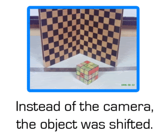Having said that, this process of "our two eyes give depth" is the fundamental concept for stereometry. But instead of "two eyes" we shifted the image instead, which theoretically, is the same thing. The A matrix from Activity 11 is shown below: Using the RQ factorization code: A=[-19.4474 18.63791 0.015063 0.031739; -5.37533 -5.41429 25.37679 -0.34856; -0.01566 -0.01596 -0.00419 1] function [R,Q]= rq(A) m = size(A,1); n = size(A,2); if n < m error(’RQ requires m <= n’) end P = mtlb_fliplr(mtlb_eye(m)); AtP = A’*P; [Q2,R2] = qr(AtP); bigperm = [P zeros(m,n-m); zeros(n-m,m) mtlb_eye(n-m)]; Q = (Q2*bigperm)’; R = (bigperm*R2*P)’; We obtain that the focal length of the camera is 5.6 mm. Moving on, we crop only the part of the image we need, we then proceed on implementing the code shown below to obtain a 3D reconstruction of the surface of the image. b = 50; f = 56; x1 = [425.83333 408.33333 447.70833 389.375 428.75 469.58333 367.5 409.79167 431.66667 453.54167 389.375 433.125 481.25 415.625 459.375 441.875 366.04167 387.91667 414.16667 459.375 478.33333 494.375 364.58333 386.45833 399.58333 412.70833 436.04167 457.91667 466.66667 475.41667 491.45833 363.125 383.54167 408.33333 436.04167 456.45833 473.95833 490]; x2 = [341.25 326.66667 363.125 304.79167 344.16667 387.91667 281.45833 323.75 344.16667 412.70833 301.875 347.08333 392.29167 326.66667 367.5 351.45833 280 300.41667 325.20833 370.41667 392.29167 411.25 280 300.41667 313.54167 323.75 347.08333 370.41667 379.16667 390.83333 409.79167 280 300.41667 322.29167 347.08333 370.41667 389.375 408.33333]; y = [172.70833 165.41667 165.41667 155.20833 156.66667 155.20833 145 145 145 145 133.33333 133.33333 133.33333 121.66667 121.66667 112.91667 117.29167 108.54167 93.958333 93.958333 105.625 114.375 89.583333 80.833333 86.666667 67.708333 56.041667 67.708333 85.208333 80.833333 91.041667 64.791667 53.125 41.458333 31.25 44.375 58.958333 69.166667]; z = b*f./((x2 - x1)); x = x1; np = 50; xp = linspace(0,1,np); yp = xp; [XP, YP] = ndgrid(xp,yp); xyz = [x' y' z']; XP = XP*38; YP = YP*38; ZP1 = eval_cshep2d(XP, YP, cshep2d(xyz)); xset("colormap", jetcolormap(64)) xbasc() plot3d1(xp, yp, ZP1, flag=[2 2 4]) posted by poy @ 7:10 PM   0 comments Tuesday, August 19, 2008 Activity 13: Photometric Stereo Continuing how image processing can be applied to our lives, we move on to photometric stereo. When we say "stereo" we usually associate the word to "music" but stereo also means having two or more images be placed together to form a 3D image, which is what we are going to do. Photometric because we use "light sources" to do this. Essentially, photometric stereo can be used to estimate the shape of the object from different locations of light sources. Processing the data from the images using the code below: (The math is included in the code, and the explanations are in the lecture notes) chdir('G:\poy\poy backup\physics\186\paper 13'); // To load the Matlab images loadmatfile('Photos.mat'); // These are the values of the light sources V1 = [0.085832 0.17365 0.98106]; V2 = [0.085832 -0.17365 0.98106]; V3 = [0.17365 0 0.98481]; V4 = [0.16318 -0.34202 0.92542]; V = [V1;V2;V3;V4]; // To produce a matrix I for intensity I1 = I1(:)'; I2 = I2(:)'; I3 = I3(:)'; I4 = I4(:)'; I = [I1;I2;I3;I4]; a = 1e-6; // This is the additive factor //g is the matrix that represents the relationship of V to I: g = inv(V'*V)*V'*I; mod = sqrt((g(1,:).*g(1,:))+(g(2,:).*g(2,:))+(g(3,:).*g(3,:))); mod = mod+a; for i = 1:3 n(i,:) = g(i,:)./mod; // To calculate for the normal vectors end nz = n(3,:)+a; dfx = -n(1,:)./nz; //Performing partial differentiation dfy = -n(2,:)./nz; z1 = matrix(dfx,128,128); // Reshaping the matrix to 128x128 z2 = matrix(dfy,128,128); int1 = cumsum(z1,2); //We use the cumsum function to perform our integration int2 = cumsum(z2,1); z = int1+int2; scf(0); plot3d(1:128, 1:128, z); // This shows the reconstruction Acknowledgments I believe I performed this activity fairly well. Thanks to Cole for helping me with the code. I think its ok to give me 10/10 neutrinos? Hehehe. posted by poy @ 1:03 AM   0 comments Monday, August 18, 2008 Activity 12: Correcting Geometric Distortions Continuing our grand pursuit of using image processing techniques to solve real-life problems, we move to removing geometric distortions from images. Geometric distortions occur because low-end cameras exist! (Hahaha! To make the life of a physicist easier, then buy high-end cameras! Kidding!) There are two kinds of distortions that may occur: a pin-cushion distortion and a barrel distortion. These distortions are better shown than meticulously explained: In the problem we will particularly solve, we are given an image of a Capiz window with an obvious barrel distortion: We "selectively select" the part where the distortion is most evident: The Capiz tiles. Then, from the image, we "envision" an "ideal" image by locating the most "undistorted" Capiz tile, obtaining its area, and assuming every tile is exactly the same. In my case I chose the tile in the 7th row, 5th column. The resulting "ideal" image is shown below: Thinking of both images (the distorted original and the ideal) as matrices that has a correlation with one another we can easily find the "transformation matrix" that links the two together (since they are obviously NOT the same! Hahaha!). Let's say the "end points" of the first Capiz tile correspond to four (x,y) pixel values, due to its distortion, these values do not correspond to the (x,y) values of the ideal image! So we equate one another to the proper matrix forms in order to get the "transformation matrix" which we would then apply to correct the distorted image! Gets? To further elaborate, I'm posting essential parts of Dr. Soriano's lecture: This was the code I used to implement the process: chdir('G:\poy\poy backup\physics\186\paper 12'); im=imread('realdistorted.jpg'); im=im2gray(im); M=[]; //I chose a wide area polygon than a relationship of just one square xi=[13; 87; 87; 16]; yi=[15; 15; 180; 181]; T=[13 14 13*14 1; 86 14 86*14 1; 86 177 86*177 1; 13 177 13*177 1]; C1=inv(T)*xi; C2=inv(T)*yi; for i=1:x for j=1:y x_im=C1(1)*i+C1(2)*j+C1(3)*i*j+C1(4); y_im=C2(1)*i+C2(2)*j+C2(3)*i*j+C2(4); if x_im>=x x_im=x; end if y_im>=y y_im=y; end M(i, j)=im(round(x_im), round(y_im)); end end scf(2); imshow(M, []); The result I obtained is best observed as a GIF file, notice the difference in the lines, they're straighter!!!: Acknowledgments This activity is HARD... no, LOOOOOONG!!! HAHAHA!!! But I did it! And I can confidently say that I am "semi-independent" in performing this activity but I really have to thank Jeric for giving me a head start in making a right code. I give myself 10/10 neutrinos! posted by poy @ 10:50 PM   0 comments		About Me Name: poy Home: Quezon City, NCR, Philippines About Me: See my complete profile Previous Post Activity 20: Neural Networks Activity 19: Linear Discriminant Analysis Activity 18: Minimum Distance Classification Activity 17: Basic Video Processing Activity 16: Parametric versus Non-Parametric Prob... Activity 15: Color Camera Processing Activity 14: Stereometry Activity 13: Photometric Stereo Activity 12: Correcting Geometric Distortions Activity 11: Camera Calibration Archives June 2008 July 2008 August 2008 September 2008 October 2008 Template by